Detailed plots with `tqec`#

The tqec library provides tools to create detailed plots of the results obtained with sinter. Below is an example of the type of plots you can generate with tqec.

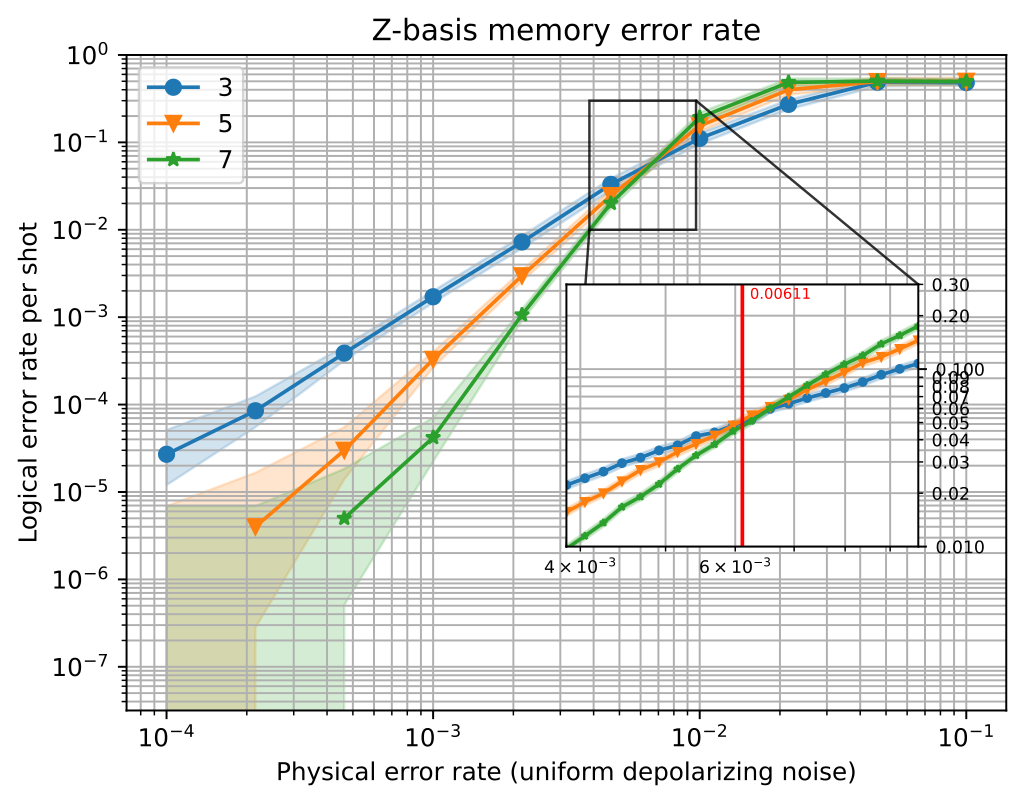
../_images/detailed_plot_memory.png — A detailed plot of the memory experiment with d = 3, 5 or 7 and an inset plot for threshold information#

This notebook will guide you through the process of creating such a plot for a basic memory experiment.

1. Create the computation#

The first step of any plot is to create the quantum computation that will be used to generate the plots. In our case, this is a memory experiment.

from tqec.gallery.memory import memory
from tqec.utils.enums import Basis

block_graph = memory(Basis.Z)
observables = block_graph.find_correlation_surfaces()

2. Perform the simulations#

Then, we need to perform multiple simulation to gather statistics to plot.

This gathering stage is split in 3 parts:

Computing general statistics over a large range of physical error-rate (e.g., \(p \in [10^{-4}, 10^{-1}]\)),
Computing an estimate of the threshold \(p_\text{thres}`\) under which increasing the code distance corrects more errors,
Computing fine statistics around the computed threshold.

First, define the parameters of our simulation.

import numpy
import sinter

from tqec.compile.convention import FIXED_BULK_CONVENTION

# Define the values of k (scaling factor) and p (physical error-rate) for which
# we want data points.
ks = list(range(1, 4))
ps = list(numpy.logspace(-4, -1, 10))

# Only use a low number of shots for demonstration purposes.
max_shots = 1_000_000
max_errors = 500

# All the data will be collected observable per observable, let's have
# data-structures to store the results
main_statistics: list[list[sinter.TaskStats]] = []
thresholds: list[float] = []
threshold_statistics: list[list[sinter.TaskStats]] = []

2.1. Gathering general statistics#

This part should be quite familiar if you already used the tqec.simulation module.

from tqec.simulation.simulation import start_simulation_using_sinter
from tqec.utils.noise_model import NoiseModel

for i, obs in enumerate(observables):
    stats = start_simulation_using_sinter(
        block_graph,
        range(1, 4),
        list(numpy.logspace(-4, -1, 10)),
        NoiseModel.uniform_depolarizing,
        manhattan_radius=2,
        convention=FIXED_BULK_CONVENTION,
        observables=[obs],
        max_shots=max_shots,
        max_errors=max_errors,
        decoders=["pymatching"],
        split_observable_stats=False,
    )
    main_statistics.append(stats[0])

2.2. Estimating the threshold#

The next step will be to have a good-enough estimation of the provided computation threshold. This threshold will help us calibrating the next step where we perform more sampling around the estimated threshold value to have a detailed view of the code behaviour near its threshold.

from math import log10

from tqec.simulation.threshold import binary_search_threshold

for obs in observables:
    threshold, _ = binary_search_threshold(
        block_graph,
        obs,
        NoiseModel.uniform_depolarizing,
        manhattan_radius=2,
        minp=10**-5,
        maxp=0.1,
        convention=FIXED_BULK_CONVENTION,
        max_shots=max_shots,
        max_errors=max_errors,
        decoders=["pymatching"],
    )
    thresholds.append(threshold)

log10_thresholds = [log10(t) for t in thresholds]
mint, maxt = min(log10_thresholds), max(log10_thresholds)
log10_threshold_bounds = (mint - 0.2, maxt + 0.2)

2.3. Gathering statistics around the threshold#

Now that we have a good estimation of the computation threshold, we can gather statistics around it.

from multiprocessing import cpu_count
from pathlib import Path

for obs in observables:
    threshold_stats = start_simulation_using_sinter(
        block_graph,
        ks,
        list(numpy.logspace(*log10_threshold_bounds, 20)),
        NoiseModel.uniform_depolarizing,
        manhattan_radius=2,
        convention=FIXED_BULK_CONVENTION,
        observables=[obs],
        num_workers=cpu_count(),
        max_shots=10_000_000,
        max_errors=5_000,
        decoders=["pymatching"],
        split_observable_stats=False,
        save_resume_filepath=Path(f"./_examples_database/detailed_plots_z.csv"),
    )
    threshold_statistics.append(threshold_stats[0])

3. Plot#

All the statistics we need should now be computed. Let’s plot!

%matplotlib inline
import matplotlib.pyplot as plt

from tqec.simulation.plotting.inset import plot_threshold_as_inset

zx_graph = block_graph.to_zx_graph()

for i, obs in enumerate(observables):
    main_stats = main_statistics[i]
    threshold = thresholds[i]
    thres_stats = threshold_statistics[i]

    fig, ax = plt.subplots()
    sinter.plot_error_rate(
        ax=ax,
        stats=main_stats,
        x_func=lambda stat: stat.json_metadata["p"],
        group_func=lambda stat: stat.json_metadata["d"],
    )
    xmin = 10 ** log10_threshold_bounds[0]
    xmax = 10 ** log10_threshold_bounds[1]
    # Note: the below values require prior knowledge about the values to look
    # for on the Y-axis.
    ymin, ymax = 1e-2, 3e-1
    plot_threshold_as_inset(
        ax,
        thres_stats,
        # Note: ymax is **before** ymin because the y axis is inversed.
        zoom_bounds=(xmin, ymax, xmax, ymin),
        threshold=threshold,
        inset_bounds=(0.5, 0.25, 0.4, 0.4),
    )
    ax.grid(which="both", axis="both")
    ax.legend()
    ax.loglog()
    ax.set_title("Z-basis memory error rate")
    ax.set_xlabel("Physical error rate (uniform depolarizing noise)")
    ax.set_ylabel("Logical error rate per shot")
    ax.set_ylim(10**-7.5, 10**0)

Detailed plots with tqec#