Three Logical CNOTs

This example demonstrates a computation involving three logical CNOT operations.

This example shows the construction and simulation results of three logical CNOT gates between three logical qubits with lattice surgery [Horsman et al.[1]].

Construction

The three CNOT gates are applied in sequence.

tqec provides builtin functions in tqec.gallery.three_cnots to construct three logical CNOT gates compressed in spacetime.

from multiprocessing import cpu_count
from pathlib import Path

import matplotlib.pyplot as plt
import numpy
import sinter

from tqec import Basis, NoiseModel, compile_block_graph
from tqec.gallery import three_cnots
from tqec.simulation.plotting.inset import plot_observable_as_inset
from tqec.simulation.simulation import start_simulation_using_sinter

graph = three_cnots()
graph.view_as_html()

The three logical CNOTs have six independent stabilizer flow generators:

• XXX -> XII

• XXI -> XIX

• XII -> XXI

• ZII -> ZII

• IZI -> ZZI

• IZZ -> IIZ

Here we show the correlation surfaces for the generators.

correlation_surfaces = graph.find_correlation_surfaces()
stab_to_surface = {s.external_stabilizer_on_graph(graph): s for s in correlation_surfaces}

XXX -> XII

graph.view_as_html(
    pop_faces_at_directions=("-Y",),
    show_correlation_surface=stab_to_surface["XXXXII"],
)

XXI -> XIX

graph.view_as_html(
    pop_faces_at_directions=("-Y",),
    show_correlation_surface=stab_to_surface["XXIXIX"],
)

XII -> XXI

graph.view_as_html(
    pop_faces_at_directions=("-Y",),
    show_correlation_surface=stab_to_surface["XIIXXI"],
)

ZII -> ZII

graph.view_as_html(
    pop_faces_at_directions=("+Z",),
    show_correlation_surface=stab_to_surface["ZIIZII"],
)

IZI -> ZZI

graph.view_as_html(
    pop_faces_at_directions=("-Y",),
    show_correlation_surface=stab_to_surface["IZIZZI"],
)

IZZ -> IIZ

graph.view_as_html(
    pop_faces_at_directions=("-Y",),
    show_correlation_surface=stab_to_surface["IZZIIZ"],
)

Example Circuit

Here we show an example circuit of three logical CNOTs with \(d=3\) surface code that is initialized and measured in the \(X\) basis. You can download the circuit here or view it in Crumble.

graph_x = three_cnots(Basis.X)
compiled_graph = compile_block_graph(graph_x)
circuit = compiled_graph.generate_stim_circuit(
    k=1, noise_model=NoiseModel.uniform_depolarizing(p=0.001)
)

Simulation

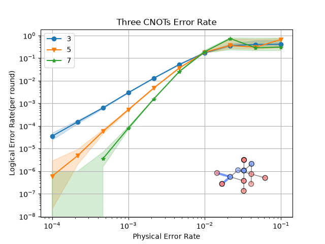
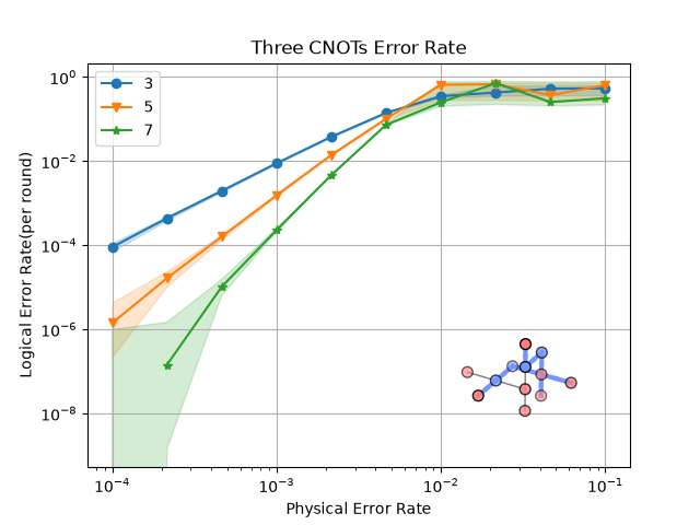
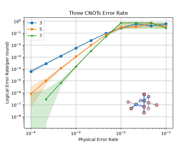
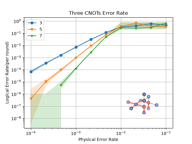
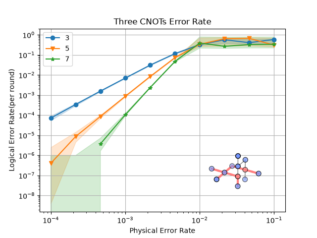
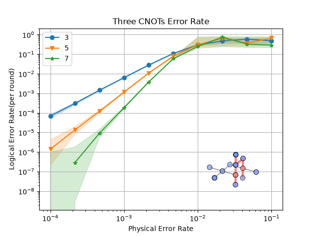
Here we show the simulation results for all six observables under a uniform depolarizing noise model.

def generate_graphs(support_observable_basis: Basis) -> None:
    """Generate the logical error-rate graphs corresponding to the provided basis."""
    block_graph = three_cnots(support_observable_basis)
    zx_graph = block_graph.to_zx_graph()

    surfaces = block_graph.find_correlation_surfaces()

    stats = start_simulation_using_sinter(
        block_graph,
        range(1, 4),
        list(numpy.logspace(-4, -1, 10)),
        NoiseModel.uniform_depolarizing,
        manhattan_radius=2,
        observables=surfaces,
        num_workers=cpu_count(),
        max_shots=1_000_000,
        max_errors=5_000,
        decoders=["pymatching"],
        save_resume_filepath=Path(
            f"../_examples_database/three_cnots_stats_{support_observable_basis.value}.csv"
        ),
        database_path=Path("../_examples_database/database.pkl"),
    )

    for i, stat in enumerate(stats):
        _, ax = plt.subplots()
        sinter.plot_error_rate(
            ax=ax,
            stats=stat,
            x_func=lambda stat: stat.json_metadata["p"],
            failure_units_per_shot_func=lambda stat: stat.json_metadata["d"],
            group_func=lambda stat: stat.json_metadata["d"],
        )
        plot_observable_as_inset(ax, zx_graph, surfaces[i])
        ax.grid(axis="both")
        ax.legend()
        ax.loglog()
        ax.set_title("Three CNOTs Error Rate")
        ax.set_xlabel("Physical Error Rate")
        ax.set_ylabel("Logical Error Rate(per round)")

Z Basis and X Basis Simulations

if __name__ == "__main__":
    generate_graphs(Basis.Z)
    generate_graphs(Basis.X)

• 
• 
• 
• 
• 
• 

References

[1]

Dominic Horsman, Austin G Fowler, Simon Devitt, and Rodney Van Meter. Surface code quantum computing by lattice surgery. New Journal of Physics, 14(12):123011, December 2012. URL: http://dx.doi.org/10.1088/1367-2630/14/12/123011, doi:10.1088/1367-2630/14/12/123011.